Thanks to Nathan at Flowing Data:

How to Make a Heatmap – a Quick and Easy Solution

How do you make a heatmap? This came from kerimcan in the FlowingData forums, and krees followed up with a couple of good links on how to do them in R. It really is super easy. Here's how to make a heatmap with just a few lines of code, but first, a short description of what a heatmap is.

The Heatmap

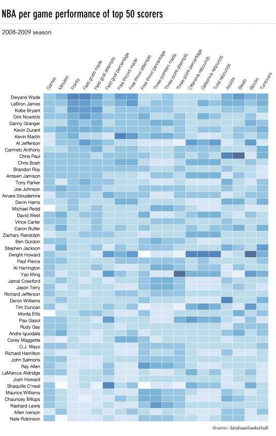
In case you don't know what a heatmap is, it's basically a table that has colors in place of numbers. Colors correspond to the level of the measurement. Each column can be a different metric like above, or it can be all the same like this one. It's useful for finding highs and lows and sometimes, patterns.

On to the tutorial.

Step 0. Download R

We're going to use R for this. It's a statistical computing language and environment, and it's free. Get it for Windows, Mac, or Linux. It's a simple one-click install for Windows and Mac. I've never tried Linux.

Did you download and install R? Okay, let's move on.

Step 1. Load the data

Like all visualization, you should start with the data. No data? No visualization for you.

For this tutorial, we'll use NBA basketball statistics from last season that I downloaded from databaseBasketball. I've made it available here as a CSV file. You don't have to download it though. R can do it for you.

I'm assuming you started R already. You should see a blank window.

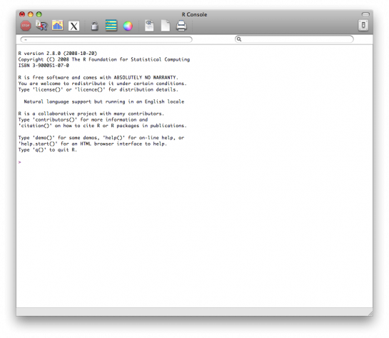
Now we'll load the data using read.csv().

nba <- read.csv("http://datasets.flowingdata.com/ppg2008.csv", sep=",")



We've read a CSV file from a URL and specified the field separator as a comma. The data is stored in nba.

Type nba in the window, and you can see the data.

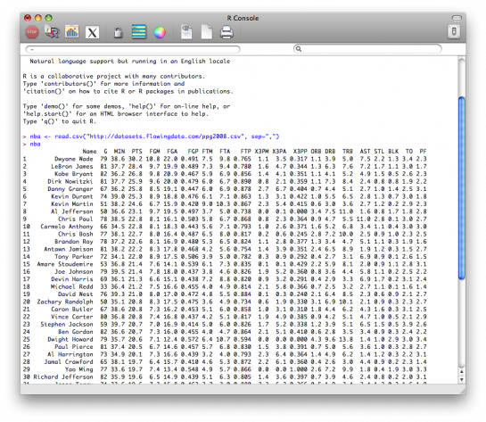
Step 2. Sort data

The data is sorted by points per game, greatest to least. Let's make it the other way around so that it's least to greatest.

nba <- nba[order(nba$PTS),]



We could just as easily chosen to order by assists, blocks, etc.

Step 3. Prepare data

As is, the column names match the CSV file's header. That's what we want.

But we also want to name the rows by player name instead of row number, so type this in the window:

row.names(nba) <- nba$Name



Now the rows are named by player, and we don't need the first column anymore so we'll get rid of it:

nba <- nba[,2:20]



Step 4. Prepare data, again

Are you noticing something here? It's important to note that a lot of visualization involves gathering and preparing data. Rarely, do you get data exactly how you need it, so you should expect to do some data munging before the visuals. Anyways, moving on.

The data was loaded into a data frame, but it has to be a data matrix to make your heatmap. The difference between a frame and a matrix is not important for this tutorial. You just need to know how to change it.

nba_matrix <- data.matrix(nba)



Step 5. Make a heatmap

It's time for the finale. In just one line of code, build the heatmap (remove the line break):

nba_heatmap <- heatmap(nba_matrix, Rowv=NA, Colv=NA,

col = cm.colors(256), scale="column", margins=c(5,10))



You should get a heatmap that looks something like this:

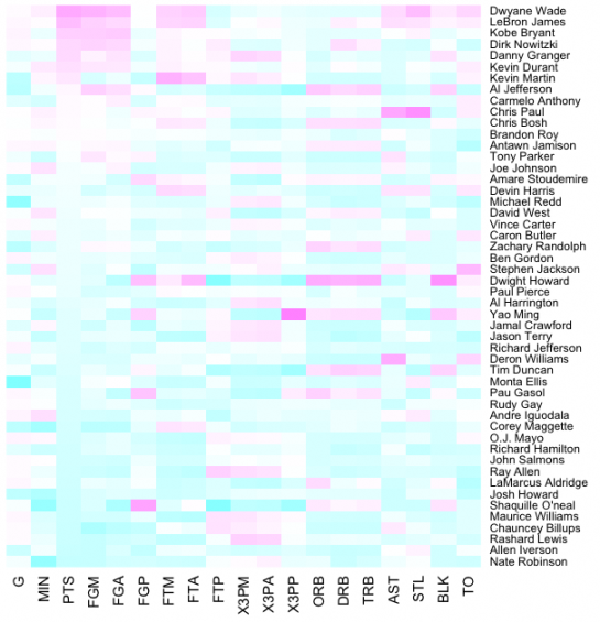
Step 6. Color selection

Maybe you want a different color scheme. Just change the argument to col, which is cm.colors(256) in the line of code we just executed. Type ?cm.colors for help on what colors R offers. For example, you could use more heat-looking colors:

nba_heatmap <- heatmap(nba_matrix, Rowv=NA, Colv=NA,

col = heat.colors(256), scale="column", margins=c(5,10))



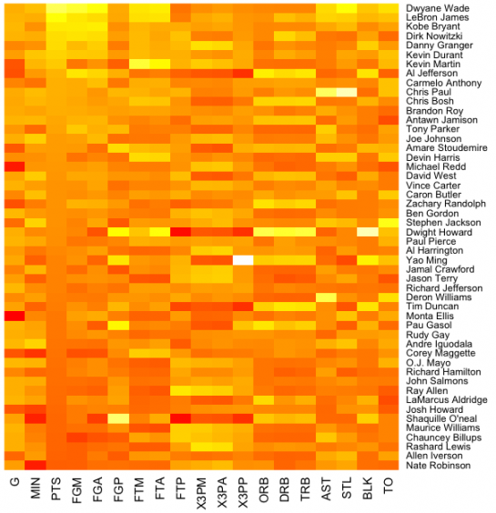
For the heatmap at the beginning of this post, I used the RColorBrewer library. Really, you can choose any color scheme you want. The col argument accepts any vector of hexidecimal-coded colors.

Step 7. Clean it up – optional

If you're using the heatmap to simply see what your data looks like, you can probably stop. But if it's for a report or presentation, you'll probably want to clean it up. You can fuss around with the options in R or you can save the graphic as a PDF and then import it into your favorite illustration software.

I personally use Adobe Illustrator, but you might prefer Inkscape, the open source (free) solution. Illustrator is kind of expensive, but you can probably find an old version on the cheap. I still use CS2. Adobe's up to CS4 already.

For the final basketball graphic, I used a blue color scheme from RColorBrewer and then lightened the blue shades, added white border, changed the font, and organized the labels in Illustrator. Voila.

Rinse and repeat to use with your own data. Have fun heatmapping.